Here, We provide Analysis and Design of Algorithms GTU Paper Solution Winter 2022. Read the Full ADA GTU paper solution given below.

Analysis and Design of Algorithms GTU Old Paper Winter 2022 [Marks : 70] : Click Here
(a) Sort the best case running times of all these algorithms in a non-decreasing
order.
LCS, Quick-Sort, Merge-Sort, Counting-Sort, Heap-Sort, Selection-Sort,
Insertion-Sort, Bucket-Sort, Strassen’s Algorithm.
Here is the non-decreasing order of the best case running times for the given algorithms:
- Bucket-Sort: O(n)
- Best case running time of bucket-sort is linear, making it the fastest in this list.
- Counting-Sort: O(n + k)
- Counting-sort has a linear best case running time, where n is the number of elements to be sorted, and k is the range of input values.
- LCS (Longest Common Subsequence): O(m * n)
- The best case running time of the LCS algorithm is quadratic, where m and n are the lengths of the input sequences.
- Insertion-Sort: O(n)
- Insertion-sort has a linear best case running time when the input is already sorted or nearly sorted.
- Merge-Sort: O(n log n)
- Merge-sort has a best case running time of n log n, which occurs when the input is already sorted or nearly sorted.
- Heap-Sort: O(n log n)
- Heap-sort has a best case running time of n log n, which occurs when the input is already sorted or nearly sorted.
- Quick-Sort: O(n log n)
- Quick-sort has a best case running time of n log n, which occurs when the input is already sorted or nearly sorted.
- Selection-Sort: O(n^2)
- Selection-sort has a quadratic best case running time, where n is the number of elements to be sorted.
- Strassen’s Algorithm: O(n^log2(7))
- Strassen’s algorithm for matrix multiplication has a best case running time of n raised to the power of log2(7), which is approximately O(n^2.807).
(b) State whether the statements are correct or incorrect with reasons.
O(f(n)) + O(f(n)) = O (2f(n))
If 3n + 5 = O(n²) , then 3n + 5 = o(n²)
- O(f(n)) + O(f(n)) = O(2f(n)) – Correct
- This statement is correct. In big O notation, when two functions are added together, the dominant term is preserved. Adding two functions with the same order of growth (denoted as O(f(n))) results in a function that is still O(f(n)). Therefore, O(f(n)) + O(f(n)) can be simplified as O(2f(n)).
- If 3n + 5 = O(n²), then 3n + 5 = o(n²) – Incorrect
- This statement is incorrect. In big O notation, the lowercase “o” notation represents a strict upper bound. If 3n + 5 is denoted as O(n²), it means that it has an upper bound of n² or less. However, it does not imply that 3n + 5 is strictly less than n², which is what the lowercase “o” notation represents. So, 3n + 5 may or may not be less than n².
(c) Explain asymptotic analysis with all the notations and its mathematical
inequalities.
Asymptotic analysis is a technique used in the analysis of algorithms to understand their behavior as the input size approaches infinity. It allows us to evaluate the efficiency and performance characteristics of an algorithm without considering the exact values or constants involved, focusing instead on how the algorithm scales with input size.
There are several notations used in asymptotic analysis to describe the upper and lower bounds of an algorithm’s running time or space complexity. The most commonly used notations are:
- Big O notation (O):
- The big O notation represents the upper bound of an algorithm’s growth rate or the worst-case scenario.
- Mathematically, O(g(n)) represents an upper bound function g(n) for a given function f(n) when there exists a positive constant c and a value n₀ such that f(n) ≤ c * g(n) for all n ≥ n₀.
- O(g(n)) provides an upper bound on the growth rate, but it does not necessarily represent the exact behavior of the function.
- Omega notation (Ω):
- The omega notation represents the lower bound of an algorithm’s growth rate or the best-case scenario.
- Mathematically, Ω(g(n)) represents a lower bound function g(n) for a given function f(n) when there exists a positive constant c and a value n₀ such that f(n) ≥ c * g(n) for all n ≥ n₀.
- Ω(g(n)) provides a lower bound on the growth rate, but it does not necessarily represent the exact behavior of the function.
- Theta notation (Θ):
- The theta notation represents the tight bound or the average-case scenario of an algorithm’s growth rate.
- Mathematically, Θ(g(n)) represents a function f(n) if and only if it satisfies both O(g(n)) and Ω(g(n)).
- Θ(g(n)) provides a precise characterization of the growth rate and represents the exact behavior of the function.
The mathematical inequalities associated with these notations are as follows:
- O(g(n)): f(n) ≤ c * g(n) for all n ≥ n₀
- Ω(g(n)): f(n) ≥ c * g(n) for all n ≥ n₀
- Θ(g(n)): c₁ * g(n) ≤ f(n) ≤ c₂ * g(n) for all n ≥ n₀
In these inequalities, f(n) represents the actual function’s growth rate, g(n) represents the bounding function, c and c₁, c₂ represent positive constants, and n₀ represents a specific threshold value from which the inequality holds true.
(a) What is the use of Loop Invariant? What should be shown to prove that an
algorithm is correct?
A loop invariant is a condition that holds true before and after each iteration of a loop in an algorithm. It is a powerful tool used in program correctness proofs and algorithm analysis. The main use of a loop invariant is to help reason about the correctness and behavior of a loop-based algorithm.
The use of a loop invariant can be summarized as follows:
- Understanding and Verification: A loop invariant helps in understanding the behavior of a loop and verifying its correctness. It serves as a guide to ensure that the loop is performing the intended operations and making progress towards the desired outcome.
- Design and Debugging: Loop invariants can aid in the design and debugging of algorithms. By formulating and maintaining a loop invariant, developers can identify and fix issues related to loop termination, boundary conditions, or incorrect intermediate results.
- Proof of Correctness: Loop invariants play a crucial role in proving the correctness of an algorithm. To demonstrate that an algorithm is correct, you typically need to show three key properties: a. Initialization: The loop invariant holds true before the first iteration of the loop. b. Maintenance: If the loop invariant holds true before an iteration, it remains true before the next iteration. c. Termination: The loop terminates, and the loop invariant, along with any post-conditions, implies the desired result.
By establishing these properties, you can demonstrate that the algorithm satisfies its specification and produces the correct output for all valid inputs.
To prove that an algorithm is correct, you typically need to show that the algorithm terminates and that it meets the required conditions specified by the problem or task. This involves demonstrating that the algorithm produces the expected output or achieves the desired goal. Loop invariants, along with other proof techniques, such as pre- and post-conditions, can be used to construct a rigorous proof of correctness.
(b) Apply LCS on sequence for pattern
To apply the Longest Common Subsequence (LCS) algorithm on a sequence to find a pattern, we need two sequences: the original sequence and the pattern we want to find within the original sequence. The LCS algorithm will then determine the longest common subsequence between the two sequences, which represents the pattern found in the original sequence.
Here is a step-by-step explanation of applying the LCS algorithm on a sequence for a given pattern:
- Define the original sequence: Identify the original sequence from which you want to find the pattern.
- Define the pattern: Determine the pattern you are searching for within the original sequence.
- Construct the LCS table: Create a table of size (n+1) x (m+1), where n is the length of the original sequence and m is the length of the pattern. Initialize all the cells of the table to 0.
- Fill in the LCS table: Iterate through the table row by row, comparing each element of the original sequence with each element of the pattern. If there is a match, increment the value of the corresponding cell in the table by 1 plus the value in the diagonal cell. If there is no match, take the maximum value from the adjacent cells above or to the left.
- Trace back the LCS: Starting from the bottom-right cell of the table, trace back the LCS by following the direction of the maximum value at each step. This can be done by moving diagonally towards the top-left corner as long as the values in the adjacent cells are decreasing. As you move, keep track of the elements that form the LCS.
- Extract the pattern: The traced back LCS will represent the pattern found within the original sequence. Extract and display the elements of the LCS to obtain the pattern.
(c) Write and explain the recurrence relation of Merge Sort.
The recurrence relation of Merge Sort can be expressed as follows:
T(n) = 2T(n/2) + O(n)
Explanation: In Merge Sort, the algorithm recursively divides the input array into two halves, sorts each half separately, and then merges the sorted halves back together. The recurrence relation captures the time complexity of the algorithm by expressing the time required to sort an array of size n in terms of the time required to sort two sub-arrays of size n/2, plus the time required for the merging step.
The recurrence relation T(n) = 2T(n/2) represents the recursive calls made by the algorithm. It states that to sort an array of size n, we make two recursive calls to sort sub-arrays of size n/2.
The term 2T(n/2) represents the time required to sort the two sub-arrays. Since the array is divided into two equal halves, each of size n/2, we recursively apply Merge Sort to each half, resulting in two recursive calls.
The term O(n) represents the time required for the merging step. After sorting the sub-arrays, the algorithm merges them together to produce a sorted array of size n. The merging process takes linear time, proportional to the size of the merged arrays.
Therefore, the overall time complexity of Merge Sort can be expressed by the recurrence relation T(n) = 2T(n/2) + O(n). This recurrence relation captures the divide-and-conquer nature of the algorithm and allows us to analyze its time complexity using techniques such as the Master Theorem or recurrence tree method.
(c) Perform the analysis of a recurrence relation T(n)= 2T (n/2) + θ(n/2) by
drawing its recurrence tree.
To analyze the given recurrence relation T(n) = 2T(n/2) + θ(n/2) by drawing its recurrence tree, we’ll break down the recursive calls and the associated costs at each level. Here’s how the recurrence tree looks:
              T(n)
           /       \
     T(n/2)       T(n/2)
     /    \       /    \
 T(n/4) T(n/4) T(n/4) T(n/4)
   .       .      .      .
   .       .      .      .
   .       .      .      .
In the recurrence tree, each level represents a recursive call, and the branching factor is 2 since we have 2T(n/2) in the recurrence relation. At each level, the input size is halved (n/2).
Now, let’s analyze the costs associated with each level of the recurrence tree:
- Level 0 (Root): The cost at the root level is θ(n/2) since it is directly given in the recurrence relation T(n) = 2T(n/2) + θ(n/2).
- Level 1: At this level, we have two subproblems of size n/2, and each subproblem incurs a cost of θ(n/2) as per the recurrence relation.
- Level 2: At this level, we have four subproblems of size n/4, and each subproblem incurs a cost of θ(n/4).
- Level 3: Similarly, at this level, we have eight subproblems of size n/8, and each subproblem incurs a cost of θ(n/8).
- The pattern continues until we reach the base case, where the subproblem size becomes 1.
To calculate the total cost, we sum up the costs at each level of the recurrence tree. The total number of levels in the tree is log₂n, as the input size is halved at each level.
Total cost = θ(n/2) + θ(n/2) + θ(n/4) + θ(n/4) + θ(n/8) + θ(n/8) + …
By summing the costs, we can simplify it as:
Total cost = θ(n/2 + n/2 + n/4 + n/4 + n/8 + n/8 + …) = θ(n(1/2 + 1/2 + 1/4 + 1/4 + 1/8 + 1/8 + …)) = θ(n)
(a) Consider the array 2,4,6,7,8,9,10,12,14,15,17,19,20. Show (without
actually sorting), how the quick sort performance will be affected with
such input.
QuickSort’s performance heavily depends on the choice of the pivot element. In the worst-case scenario, if the pivot is consistently chosen as the smallest or largest element in the array, QuickSort’s efficiency can degrade, resulting in poor performance.
In the given array [2, 4, 6, 7, 8, 9, 10, 12, 14, 15, 17, 19, 20], if the QuickSort algorithm consistently chooses the first or last element as the pivot, the partitioning step will divide the array into two sub-arrays with highly imbalanced sizes. Let’s consider the case where the pivot is chosen as the first element (2):
- First partitioning step: The array is partitioned into two sub-arrays:
- [2] (elements less than or equal to the pivot)
- [4, 6, 7, 8, 9, 10, 12, 14, 15, 17, 19, 20] (elements greater than the pivot)
- Second partitioning step: The second sub-array is further divided:
- [4, 6, 7, 8, 9, 10, 12, 14, 15, 17, 19, 20] (elements greater than the pivot)
- (empty sub-array)
At each step, the pivot element separates the array into one smaller sub-array and one larger sub-array. This imbalanced partitioning results in a skewed recursion tree, where the smaller sub-array has only one element while the larger sub-array contains the remaining elements. Consequently, QuickSort will exhibit poor performance, approaching the worst-case time complexity of O(n^2).
It’s important to note that this worst-case scenario is specific to the choice of pivot and the given input array. QuickSort’s average-case time complexity is O(n log n), and in most cases, it performs efficiently. To mitigate the worst-case scenario, various techniques can be employed, such as choosing a random pivot, using a median-of-three pivot selection, or implementing an optimized version of QuickSort like “IntroSort.”
(b) “A greedy strategy will work for fractional Knapsack problem but not for
0/1″, is this true or false? Explain.
This statement is true. A greedy strategy can work for the Fractional Knapsack problem but not for the 0/1 Knapsack problem.
The Fractional Knapsack problem involves selecting items from a set with certain weights and values, with the goal of maximizing the total value while considering the weight constraint of the knapsack. The key difference between the Fractional Knapsack problem and the 0/1 Knapsack problem lies in the constraint on item selection:
- Fractional Knapsack problem: In this problem, we can take fractions of items, meaning we can select a fraction of an item’s weight to maximize the total value. This allows us to employ a greedy strategy based on the item’s value-to-weight ratio. We prioritize selecting items with a higher value-to-weight ratio, as it provides the best value for the weight. This strategy ensures an optimal solution.
- 0/1 Knapsack problem: In this problem, we can only take items in their entirety (either include an item completely or exclude it). We cannot take fractional parts of items. This constraint makes the problem more challenging and prevents a simple greedy strategy from guaranteeing an optimal solution. A greedy strategy based solely on the value-to-weight ratio can lead to suboptimal solutions because it does not consider the full weight constraint. It is possible that a lower-value item with a lower weight can be chosen instead of a higher-value item that exceeds the weight limit, resulting in a suboptimal solution.
To solve the 0/1 Knapsack problem optimally, dynamic programming algorithms are commonly employed, which consider all possible combinations and evaluate their values and weights to determine the optimal solution. The dynamic programming approach ensures that the weight constraint is satisfied while maximizing the total value.
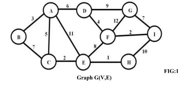
(c) Apply Kruskal’s algorithm on the given graph and step by step generate
the MST.
OR
(a) Consider an array of size 2048 elements sorted in non-decreasing order.
Show how the Binary Search will perform on this size by analysis of its
recurrence relation. Derive the running time.
To analyze the performance of binary search on an array of size 2048, we can derive its recurrence relation and then determine its running time.
Binary search is a divide-and-conquer algorithm that repeatedly divides the search space in half until the target element is found or the search space is exhausted. Here’s how we can analyze its recurrence relation:
- Let’s denote the size of the array at each step as n.
- In each step of binary search, we divide the array in half, resulting in two subproblems of size n/2.
- We compare the target element with the middle element of the array to determine if the target is in the left or right half.
- If the target is in the left half, we recursively perform binary search on the left subproblem of size n/2.
- If the target is in the right half, we recursively perform binary search on the right subproblem of size n/2.
- The base case occurs when the size of the array becomes 1, and we either find the target or conclude that it is not present.
Now, let’s derive the recurrence relation for the running time of binary search:
T(n) = T(n/2) + c
Here, T(n) represents the running time of binary search on an array of size n, and c represents the constant time taken for comparisons and other operations within each recursive call.
Using the recurrence relation, we can determine the running time by solving it recursively:
T(n) = T(n/2) + c = T(n/4) + c + c = T(n/8) + c + c + c = T(n/16) + c + c + c + c = …
This pattern continues until we reach the base case when n = 1.
At each step, we perform a constant amount of work (c) to divide the array in half and compare the target with the middle element. Since we divide the array in half at each step, the number of steps required to reach the base case is log₂n.
Therefore, the total running time of binary search on an array of size 2048 is:
T(n) = c + c + c + … + c (log₂n times) = c * log₂n
(b) Explain the steps of greedy strategy for solving a problem.
The greedy strategy is an algorithmic approach that involves making locally optimal choices at each step with the aim of finding a global optimum. It follows a set of steps to solve a problem. Here are the general steps of the greedy strategy:
- Understand the problem: Gain a clear understanding of the problem statement, constraints, and the desired objective. Identify the specific problem that can be solved using a greedy approach.
- Define the objective function: Determine the objective function or criteria that need to be optimized or maximized. This could be the maximum value, minimum cost, maximum efficiency, etc.
- Identify the greedy choice: Determine the best local choice at each step that seems optimal. This involves identifying the element, action, or decision that maximizes the objective function at the current step.
- Develop the greedy algorithm: Formulate the algorithm based on the identified greedy choices. This involves defining the data structures, variables, and control flow to implement the greedy approach.
- Validate the greedy choice: Ensure that the greedy choice made at each step is valid and does not violate any constraints. Verify that the greedy choice leads to a feasible solution.
- Iterate until a solution is found: Apply the greedy choice iteratively to make successive decisions until a solution is found. Each decision affects the problem space and narrows down the solution space.
- Verify the solution: Once a solution is obtained, validate it to ensure it meets all the desired criteria and constraints. Check if the solution is globally optimal or satisfies the objective function.
It’s important to note that the greedy strategy does not guarantee an optimal solution for all problems. It may provide a suboptimal solution or fail to find a feasible solution in some cases. However, when the greedy strategy is applicable and works effectively, it offers simplicity and efficiency in solving problems.
(c) Apply Prim’s algorithm on the given graph in Q.3 (C) FIG:1 Graph
G(V,E) and step by step generate the MST.
(a) Given is the S-table after running Chain Matrix Multiplication algorithm.
Calculate the parenthesized output based on
PRINT_OPTIMAL_PARENTHESIS algorithm. Assume the matrix are
names from A1, A2, ….,An
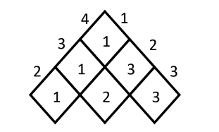
Based on the provided S-table from the Chain Matrix Multiplication algorithm, we can use the PRINT_OPTIMAL_PARENTHESIS algorithm to calculate the parenthesized output. Here’s how it can be done:
To calculate the parenthesized output, we start from the top-right corner of the S-table and recursively follow the optimal parenthesization.
- Starting from the top-right cell, if the value in the cell is denoted by S[i][j], we know that the optimal multiplication for matrices A[i] to A[j] lies between A[i] and A[S[i][j]].
- If S[i][j] = k, it means that the optimal multiplication occurs between A[i] to A[k] and A[k+1] to A[j].
- We recursively apply the PRINT_OPTIMAL_PARENTHESIS algorithm for each half until we reach the base case.
Applying this algorithm to the given S-table:
- From the top-right cell (S[1][3]), we have S[1][3] = 2, which means the optimal multiplication occurs between A[1] to A[2] and A[3].
- Recursively, for the first half (A[1] to A[2]), we have S[1][2] = 1, indicating that the optimal multiplication occurs between A[1] and A[1].
- Recursively, for the second half (A[3]), there is no further split as it contains only one matrix.
Putting it all together, the parenthesized output for the optimal multiplication order is:
(A1(A2A3))
This means that we first multiply matrices A2 and A3, and then multiply the result with A1.
(b) Explain states, constraints types of nodes and bounding function used by
backtracking and branch and bound methods.
Backtracking and branch and bound are algorithmic techniques used for problem-solving. They both involve exploring the solution space of a problem, but they employ different strategies to find the optimal solution.
- Backtracking:
- States: Backtracking involves maintaining a set of states that represent the partial solutions being explored. Each state represents a partial assignment or configuration of the problem.
- Constraints: Backtracking utilizes constraints to determine if a particular partial solution is valid or violates any conditions. These constraints help in making decisions during the search process, allowing the algorithm to backtrack and explore alternative paths when a constraint is violated.
- Types of Nodes: In backtracking, nodes represent different states or partial solutions in the search space. Each node corresponds to a decision point where choices are made to progress towards the solution.
- Bounding Function: Backtracking may use a bounding function to perform pruning and eliminate certain nodes from further exploration. The bounding function helps in determining if a particular node or state is promising enough to continue the search or if it can be pruned based on some criteria. This can help reduce the search space and improve the efficiency of the algorithm.
- Branch and Bound:
- States: Branch and bound also involves maintaining a set of states representing partial solutions. Each state represents a partial assignment or configuration of the problem, similar to backtracking.
- Constraints: Like backtracking, branch and bound utilize constraints to ensure that partial solutions are valid. Constraints guide the search process and help in making decisions at each level of the search tree.
- Types of Nodes: In branch and bound, nodes represent various states or partial solutions in the search space, similar to backtracking. Each node corresponds to a decision point where choices are made to explore different paths.
- Bounding Function: Branch and bound utilizes a bounding function to perform pruning and optimize the search process. The bounding function provides an upper or lower bound on the objective function or cost associated with a particular node or partial solution. Based on these bounds, the algorithm can prune certain branches or subproblems that are deemed non-promising or suboptimal, reducing the search space and improving efficiency.
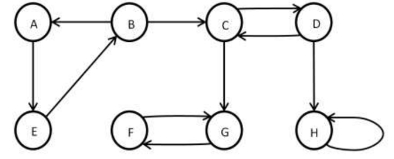
(c) Apply the algorithm to find strongly connected components from the
given graph.
OR
(a) Consider a Knapsack with maximum weight capacity M is 7, for the three
objects with value <3, 4, 5> with weights <2, 3, 4> solve using dynamic
programming the maximum value the knapsack can have.
To solve the knapsack problem using dynamic programming, we can create a table to store the maximum value that can be achieved for each combination of object and weight capacity. Here’s how we can solve it for the given scenario:
- Create a table with (n + 1) rows and (M + 1) columns, where n is the number of objects and M is the maximum weight capacity of the knapsack. Initialize all cells to 0.
- Iterate through each object:
- For each object i from 1 to n, calculate its value and weight.
- Iterate through each weight capacity w from 1 to M.
- If the weight of the object (weights[i-1]) is greater than the current weight capacity w, copy the value from the cell above (table[i-1][w]).
- Otherwise, calculate the maximum value between taking the object (value[i-1] + table[i-1][w – weights[i-1]]) and not taking the object (table[i-1][w]).
- Store the maximum value in the current cell (table[i][w]).
- The maximum value of the knapsack can be found in the bottom-right cell of the table (table[n][M]).
Applying the dynamic programming approach to the given scenario:
Object values: <3, 4, 5> Object weights: <2, 3, 4> Maximum weight capacity: M = 7
The table will look like this:
      | 0 | 1 | 2 | 3 | 4 | 5 | 6 | 7 |
-------------------------------------
Obj 0 | 0 | 0 | 0 | 0 | 0 | 0 | 0 | 0 |
Obj 1 | 0 | 0 | 3 | 3 | 3 | 3 | 3 | 3 |
Obj 2 | 0 | 0 | 3 | 4 | 4 | 7 | 7 | 7 |
Obj 3 | 0 | 0 | 3 | 4 | 5 | 7 | 8 | 9 |
The maximum value the knapsack can have is 9, which is obtained by including objects with values 3, 4, and 5, and weights 2, 3, and 4 respectively.
Please note that in the table, the row and column indices are shifted by 1 compared to the object and weight indices.
(b) Explain the Minimax principle and show its working for simple tic-tac-toe game
playing.
The Minimax principle is a decision-making strategy used in game theory and artificial intelligence. It is commonly applied in games with perfect information, such as tic-tac-toe, chess, or checkers. The goal of the Minimax principle is to determine the best possible move for a player by considering all possible future game states and their outcomes.
The Minimax principle works by assuming that both players in the game are playing optimally and trying to maximize their own gains while minimizing their opponent’s gains. It assumes that the opponent will always make the best move for themselves. The Minimax algorithm recursively evaluates all possible moves from the current game state and assigns a value to each move based on its potential outcome.
Here’s how the Minimax principle can be applied to a simple tic-tac-toe game:
- Evaluate the current game state:
- If the game state is a terminal state (win, loss, or draw), assign a value of +1 for a win, -1 for a loss, or 0 for a draw.
- If the game state is not terminal, proceed to the next step.
- Generate all possible moves:
- Generate all legal moves that the current player can make from the current game state.
- Evaluate each possible move:
- For each possible move, recursively apply the Minimax algorithm by assuming the opponent will play optimally.
- Assign a value to each move based on the outcomes of the subsequent game states obtained by making that move.
- Determine the best move:
- If it is the current player’s turn, choose the move with the highest value.
- If it is the opponent’s turn, choose the move with the lowest value.
- Repeat steps 1-4 until a terminal state is reached.
By following this process, the Minimax algorithm explores all possible moves and their outcomes, eventually selecting the optimal move for the current player. In tic-tac-toe, the Minimax algorithm can help a player determine the best move to make at each turn, leading to optimal gameplay and maximizing their chances of winning or achieving a draw against an opponent playing optimally.
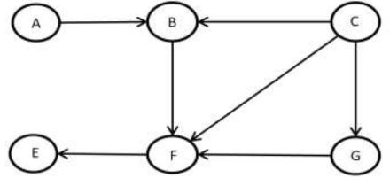
(c) Given is the DAG, apply the algorithm to perform topological sort and
show the sorted graph.
(a) When can we say that a problem exhibits the property of Optimal Sub-
structure?
A problem exhibits the property of Optimal Substructure when an optimal solution to the problem can be constructed from optimal solutions to its subproblems. In other words, the problem can be broken down into smaller subproblems, and the optimal solution to the overall problem can be found by combining the optimal solutions of the subproblems.
Formally, a problem has Optimal Substructure if it satisfies the following condition:
For a problem P, let’s say we have an optimal solution S to P. If we break down P into smaller subproblems and find optimal solutions for each subproblem, then we can combine these optimal solutions to construct an optimal solution for P.
Optimal Substructure is a key property in dynamic programming, as it allows us to apply the technique of solving a problem recursively and building up the solutions of smaller subproblems to solve the larger problem efficiently.
To determine if a problem exhibits Optimal Substructure, we need to analyze the problem and identify if it can be divided into subproblems that have independent optimal solutions and if the optimal solution of the larger problem can be derived from the optimal solutions of the subproblems.
(b) Create an example of string P of length 7 such that, the prefix function of KMP
string matcher returns π[5] = 3, π[3] = 1 and π[1] = 0
To create an example string P that satisfies the given conditions, we can construct a string where the prefix function values match the specified values.
Let’s consider the string P = “ABCDABC”.
The prefix function (π) of P is as follows: π[1] = 0 π[2] = 0 π[3] = 0 π[4] = 1 π[5] = 3 π[6] = 0 π[7] = 0
In this example, π[5] = 3 means that the longest proper prefix of the substring P[1:5] (which is “ABCDA”) that is also a suffix has a length of 3. Similarly, π[3] = 1 means that the longest proper prefix of the substring P[1:3] (which is “ABC”) that is also a suffix has a length of 1. Finally, π[1] = 0 means that there is no proper prefix of the substring P[1] (which is “A”) that is also a suffix.
Thus, the string P = “ABCDABC” satisfies the given conditions for the prefix function values in KMP string matching.
(c) Explain the 3SAT problem and show that it is NP Complete.
The 3SAT problem is a well-known problem in computer science and computational complexity theory. It is a decision problem that asks whether there exists a satisfying assignment for a given Boolean formula in Conjunctive Normal Form (CNF), where each clause contains exactly three literals connected by logical OR operators and each literal is a variable or its negation.
To show that the 3SAT problem is NP-complete, we need to demonstrate two things:
- The 3SAT problem is in the NP class: This means that given a proposed solution (a satisfying assignment), we can verify its correctness in polynomial time. For the 3SAT problem, we can check if a given assignment satisfies each clause of the CNF formula by evaluating the truth value of each clause. This verification process can be done in polynomial time, making the problem part of NP.
- The 3SAT problem is NP-hard: This means that any problem in the NP class can be reduced to the 3SAT problem in polynomial time. In other words, if we can efficiently solve the 3SAT problem, we can solve any problem in NP efficiently. To establish this, we can perform a reduction from a known NP-complete problem, such as the Boolean Satisfiability Problem (SAT), to the 3SAT problem. This reduction shows that an instance of SAT can be transformed into an equivalent instance of 3SAT in polynomial time, preserving the satisfiability of the formula.
By satisfying both conditions, we can conclude that the 3SAT problem is NP-complete. This means that it is among the hardest problems in the class NP, and if a polynomial-time algorithm exists for the 3SAT problem, it would imply that P = NP, a major open question in computer science.
OR
(a) Explain Over-lapping Sub-problem with respect to dynamic
programming.
In dynamic programming, the concept of overlapping subproblems refers to the situation where the solution to a larger problem can be efficiently computed by breaking it down into smaller subproblems, and these subproblems share common sub-subproblems. As a result, the same subproblems are repeatedly solved multiple times instead of being recomputed from scratch. Overlapping subproblems are a key characteristic of many problems that can be solved using dynamic programming techniques.
To illustrate the concept of overlapping subproblems, let’s consider the Fibonacci sequence. The Fibonacci sequence is defined as follows: F(0) = 0, F(1) = 1, and for n ≥ 2, F(n) = F(n-1) + F(n-2). We can compute the nth Fibonacci number using a dynamic programming approach:
function Fibonacci(n):
    if n <= 1:
        return n
    else:
        memo = array of size n+1
        memo[0] = 0
        memo[1] = 1
        for i from 2 to n:
            memo[i] = memo[i-1] + memo[i-2]
        return memo[n]
In this approach, we use an array memo to store the computed Fibonacci numbers. By starting from the base cases (F(0) and F(1)) and iteratively computing subsequent Fibonacci numbers up to n, we avoid redundant calculations. Without using dynamic programming, calculating each Fibonacci number would require recomputing the entire sequence from scratch, resulting in exponential time complexity.
The overlapping subproblems occur because when calculating F(n), we need the previously computed Fibonacci numbers F(n-1) and F(n-2), which are subproblems themselves. By storing the solutions to these subproblems in the memo array, we eliminate the need to recompute them and achieve significant performance improvements.
(b) Show that if all the characters of pattern P of size m are different, the naïve string
matching algorithm can perform better with modification. Write the modified
algorithm that performs better than O(n.m).
If all the characters of the pattern P of size m are different, we can make a modification to the naïve string matching algorithm to improve its performance.
The naïve string matching algorithm compares the pattern P with each possible substring of the text T of size m. In each comparison, it checks if the characters of P match the corresponding characters of the substring in T. If a mismatch is found, it moves to the next substring and repeats the process.
However, if all characters of P are different, we can take advantage of this uniqueness to optimize the algorithm. Instead of comparing character by character, we can directly jump to the next possible substring by considering only the last character of the substring.
Here’s the modified algorithm:
function ModifiedNaiveStringMatching(text T, pattern P):
    n = length(T)
    m = length(P)
    i = 0

    while i <= n - m:
        j = m - 1
        while j >= 0 and P[j] == T[i + j]:
            j = j - 1

        if j == -1:
            // Match found at index i
            return i

        // Move to the next possible substring
        i = i + max(1, m - j - 1)

    // No match found
    return -1
In this modified algorithm, we start comparing the characters of P with the corresponding characters of the substring in T from the rightmost end. If a mismatch is found, instead of moving one character at a time, we calculate the number of positions we can safely skip. This skipping value is given by max(1, m - j - 1), where j represents the index of the mismatched character.
(c) Explain with example, how the Hamiltonian Cycle problem can be used to solve
the Travelling Salesman problem.
The Hamiltonian Cycle problem and the Traveling Salesman problem are closely related. In fact, the Traveling Salesman problem (TSP) can be reduced to the Hamiltonian Cycle problem (HCP) in order to solve it.
The Hamiltonian Cycle problem asks whether a given graph contains a cycle that visits every vertex exactly once. The Traveling Salesman problem, on the other hand, asks for the shortest possible route that visits every city once and returns to the starting city.
To solve the TSP using the HCP, we can construct a graph from the given cities where each city is represented by a vertex. We then add edges between every pair of cities, and assign weights to the edges representing the distances between the cities.
For example, consider the following cities and their distances:
Cities: A, B, C Distances: AB = 3, AC = 4, BC = 2
We can construct the following complete graph:
      A
    /   \
   3     4
  /       \
 B -- 2 -- C
Now, if we find a Hamiltonian Cycle in this graph, it represents a route that visits every city exactly once. By summing up the weights of the edges in the Hamiltonian Cycle, we get the total distance of the route.
In our example, if the Hamiltonian Cycle is A-B-C-A, the total distance would be 3 + 2 + 4 = 9. This represents the shortest possible route that visits all cities once and returns to the starting city.
“Do you have the answer to any of the questions provided on our website? If so, please let us know by providing the question number and your answer in the space provided below. We appreciate your contributions to helping other students succeed.